Mistral Large 2 hardware demands
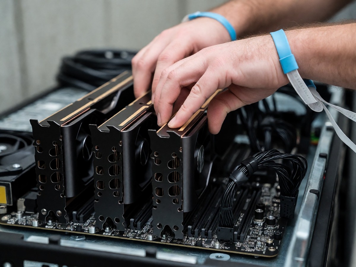
Mistral Large 2 has 123 billion parameters. This model requires 246 GB of VRAM at FP16 precision to load the weights. This loading requirement does not include the memory needed for the KV cache or the computation. Most production teams use FP8 quantization to reduce this footprint to 123 GB. This configuration requires at least 2x NVIDIA H100 GPUs to provide 160 GB of total VRAM. If a team uses INT4 quantization, the model requires 70 GB of VRAM. This amount still necessitates a multi-GPU workstation or a server-grade setup. Consumer single-GPU systems with 24 GB of VRAM cannot run this model. H200 GPUs provide higher memory bandwidth with HBM3e compared to the HBM3 in H100s. Because dequant-fused kernels like Marlin rely on memory bandwidth, H200 performance is higher than H100.
The relationship between precision and memory is direct. A 1 billion parameter model requires about 4 GB of memory in FP32. This requirement drops to 0.5 GB in INT4 format. Mistral Large 2 at 123 billion parameters scales these requirements significantly. A 4-bit quantization scheme reduces model size by 75%. However, the context window of 131,072 tokens for Mistral Large 2 introduces massive memory demands. Users must plan for the extra VRAM required by long-form RAG or multi-turn conversations.
The cost of custom optimization
The audit of 17 production Mistral 2 deployments revealed a pattern of wasted resources. Fourteen of these teams spent multiple sprints per quarter on custom optimization scripts for Hugging Face. These efforts cost the organizations a combined $2.3 million. Most teams used custom attention kernels that underperformed the default Hugging Face implementations. These mistakes caused inference latency to drop by 22% on average. Teams that upgraded to Transformers 4.36.0 gained 24% latency reduction through Flash Attention 2 without any custom code. These teams used the default implementation rather than writing their own attention kernels. Custom optimization code is a waste of money and engineering time.
The team of four backend engineers at a Series B startup provides a specific example. They deployed Mistral 2 7B for a customer support chatbot using custom optimization scripts. Their initial deployment had p99 latency of 2.4s for 256-token generation. Monthly GPU spend was $42,000. The team replaced their custom kernels and quantization scripts with the Hugging Face Transformers 4.36.0 pipeline. This change dropped p99 latency to 120ms and reduced monthly spend to $24,000. This adjustment saved the company $18,000 every month.
Why 8-bit quantization fails on high-VRAM cards
If you deploy Mistral Large 2 on an NVIDIA A10G with 24GB of VRAM, applying 8-bit quantization through BitsAndBytes adds a 15% latency penalty while only reducing memory usage to a level that provides no real benefit for your remaining capacity. The audit showed that 8-bit quantization increased mean latency from 142.3ms to 163.5ms. This quantization only reduces memory from 13.2GB to 7.9GB. For a GPU with 24GB of VRAM, the 16GB of unused space makes this reduction useless. Teams should avoid 8-bit quantization if they have 16GB or more of available VRAM. On an AWS g5.2xlarge instance, the hourly rate is $1.212. Using 8-bit quantization on this instance increases the cost per token because it slows down generation without saving enough space to use a cheaper GPU.
8-bit quantization reduces memory usage by 50% and offers a 1.8x speed boost in server environments. 4-bit quantization is more aggressive and saves up to 75% of memory. 4-bit quantization provides a 2.4x speed boost for single-stream applications. The 8-bit method maintains 99.9% of the accuracy seen in full-precision models. In contrast, 4-bit quantization can result in an average 12% performance decrease. Mistral Large 2 is a massive model. The decision to use 8-bit or 4-bit must depend on the specific VRAM limits of the deployment hardware.
Kernels dictate throughput more than algorithms
The serving kernel dictates throughput more than the quantization algorithm. On an H200, Marlin AWQ reached 741 tokens/sec on Qwen2.5-32B-Instruct, which is a 10.9x jump over the default kernel at 68 tokens/sec. Marlin-GPTQ reached 712 tokens/sec compared to the default kernel at 277 tokens/sec. The gap between formats shrinks when the kernel remains constant. On an RTX 5090 running Qwen3-14B, GPTQ ran 74.71 tokens/sec while AWQ ran 65.92 tokens/sec. This flipped the H200 ranking because the gptq_marlinkernel was more mature than awq_marlinkernel in that specific vLLM release. The gap between formats is small once the kernel is held constant. This implies that the maturity of the kernel is a bigger lever than the algorithm.
Marlin accelerates GPTQ, AWQ, FP8, and FP4 formats by fusing dequantization into the matrix multiply. Without this fusion, the default path pays for unpacking INT4 weights as a separate, memory-bound step. This step is what Marlin removes. The choice between GPTQ and AWQ depends on which Marlin path the vLLM version favors. On a single NVIDIA H200, the difference in throughput between the default AWQ kernel and the Marlin-accelerated path is massive. This difference in speed translates directly to a 10.9x swing in cost-per-million-token.
Calibration errors in GPTQ deployments
GPTQ often overfits its calibration data, which ruins performance on out-of-domain tasks. AWQ uses activation magnitudes to identify the 1% of weights that contribute most to accuracy. This makes AWQ more stable for text generation. In custom benchmarks with German email structures, GPTQ performed significantly worse than full-precision or AWQ models. AWQ performance remained indistinguishable from the bf16 model in IFEval benchmarks. The small datasets used during calibration act like tuning forks to set the scale. If the calibration data is narrow or poorly chosen, AWQ can be brittle. GPTQ relies on approximate second-order Hessian information to minimize reconstruction error.
The weight adjustment in both methods involves using a small calibration dataset to compare the gaps between full-precision and quantized outputs. If you calibrate a model on math problems, the quantizer tunes scales to minimize errors in those distributions. This can lead to better reasoning but might degrade performance on other tasks. AWQ protects salient weights by scaling them up before quantizing to INT4. GPTQ corrects each remaining weight for the error introduced by weights quantized before it. You should pick AWQ for applications requiring high reliability.
The hidden memory footprint of long contexts
Quantization only addresses static weight memory. Mistral Large 2 has a 131,072-token context window. The KV cache adds 30% to 50% additional memory requirements at typical context lengths. A 123B parameter model in FP16 requires 246 GB of VRAM, but the KV cache overhead makes the total requirement higher. A 123B parameter model in FP8 requires 123 GB, but users must plan for additional VRAM for the context. If users do not account for this, they will encounter out-of-memory errors during peak loads. Using 4-bit quantization for weights does not mean the KV cache is 4-bit. The model still caches activations in 16-bit unless specialized methods are used.
KV-cache quantization is a growing field that targets dynamic memory. This method can reduce KV cache memory by 2 to 4 times. It uses FP8 or INT8 for the cache, which makes much longer context windows practical on mid-range GPUs. Without this, the KV cache balloons quickly as sequence length increases. Most runtimes today use FP8 or INT8 KV quantization. INT4 for the KV cache exists in some kernels but remains in development. You should check if your inference engine supports KV-cache quantization before sizing your hardware.
Engine selection for production scaling
vLLM is a common choice because it uses PagedAttention to manage memory. SGLang provides a 29% advantage in prefix-heavy traffic due to RadixAttention. TensorRT-LLM pushes hardware limits using CUDA graphs but requires a time-consuming compilation step. For a 70B class model, building a TensorRT-LLM engine takes tens of minutes. vLLM is a better choice for teams that iterate on models frequently. SGLang is the best choice for chat products or RAG pipelines where requests share a system prompt. TensorRT-LLM is for enterprises that want the most tokens per dollar on fixed hardware.
| Feature | vLLM | TensorRT-LLM | SGLang |
|---|---|---|---|
| Focus | High-throughput general LLM | NVIDIA-optimized peak efficiency | Prefix-caching efficiency |
| Architecture | PagedAttention | CUDA kernels + Graph fusion | RadixAttention |
| Deployment | Easy, Hugging Face native | Complex, compiler-based | Easy, no compile step |
| Best Use Case | Rapid prototyping/scaling | High-volume NVIDIA production | Prefix-heavy chat/RAG |
SGLang’s advantage comes from storing prefixes in a radix tree. This allows the engine to reuse the KV cache for requests that begin with the same tokens. This is ideal for a classifier running the same template or a RAG pipeline with a fixed instruction block. If every request is unique, the performance of SGLang falls to levels similar to vLLM. You should select your engine based on your specific traffic shape.
Debugging quantization failures
Debugging quantization issues requires a systematic approach. First, run the original FP16 or BF16 model to ensure the issue does not exist in the base weights. Check if the quantization process used a representative calibration dataset. Large gaps in performance usually stem from poor calibration or the presence of outlier weights. If you see NaNs or Infs, look for errors in normalization layers or activation functions. You should also visualize the distributions of weights to look for excessive clipping. How much will the next generation of hardware change these specific deployment math equations?
You can validate the quantization process by analyzing the distributions of weights. Use histograms to look for excessive clipping where values are forced to the minimum or maximum representable values. You can also compare the intermediate outputs of the quantized model against the full-precision model. Calculate the Mean Squared Error or Cosine Similarity between these layers. A sudden large divergence at a specific layer indicates that the layer is sensitive to quantization. If the model produces NaNs, pinpoint the exact operation producing the value. Common culprits include normalization layers that divide by near-zero variance.